UPDATE: If you're interested in learning pandas from a SQL perspective and would prefer to watch a video, you can find video of my 2014 PyData NYC talk here.
This is part three of a three part introduction to pandas, a Python library for data analysis. The tutorial is primarily geared towards SQL users, but is useful for anyone wanting to get started with the library.
- Part 1: Intro to pandas data structures, covers the basics of the library's two main data structures - Series and DataFrames.
- Part 2: Working with DataFrames, dives a bit deeper into the functionality of DataFrames. It shows how to inspect, select, filter, merge, combine, and group your data.
- Part 3: Using pandas with the MovieLens dataset, applies the learnings of the first two parts in order to answer a few basic analysis questions about the MovieLens ratings data.
Using pandas on the MovieLens dataset
To show pandas in a more "applied" sense, let's use it to answer some questions about the MovieLens dataset. Recall that we've already read our data into DataFrames and merged it.
# pass in column names for each CSV
u_cols = ['user_id', 'age', 'sex', 'occupation', 'zip_code']
users = pd.read_csv('ml-100k/u.user', sep='|', names=u_cols,
                    encoding='latin-1')

r_cols = ['user_id', 'movie_id', 'rating', 'unix_timestamp']
ratings = pd.read_csv('ml-100k/u.data', sep='\t', names=r_cols,
                      encoding='latin-1')

# the movies file contains columns indicating the movie's genres
# let's only load the first five columns of the file with usecols
m_cols = ['movie_id', 'title', 'release_date', 'video_release_date', 'imdb_url']
movies = pd.read_csv('ml-100k/u.item', sep='|', names=m_cols, usecols=range(5),
                     encoding='latin-1')

# create one merged DataFrame
movie_ratings = pd.merge(movies, ratings)
lens = pd.merge(movie_ratings, users)
What are the 25 most rated movies?
most_rated = lens.groupby('title').size().sort_values(ascending=False)[:25]
most_rated
title
Star Wars (1977)                             583
Contact (1997)                               509
Fargo (1996)                                 508
Return of the Jedi (1983)                    507
Liar Liar (1997)                             485
English Patient, The (1996)                  481
Scream (1996)                                478
Toy Story (1995)                             452
Air Force One (1997)                         431
Independence Day (ID4) (1996)                429
Raiders of the Lost Ark (1981)               420
Godfather, The (1972)                        413
Pulp Fiction (1994)                          394
Twelve Monkeys (1995)                        392
Silence of the Lambs, The (1991)             390
Jerry Maguire (1996)                         384
Chasing Amy (1997)                           379
Rock, The (1996)                             378
Empire Strikes Back, The (1980)              367
Star Trek: First Contact (1996)              365
Back to the Future (1985)                    350
Titanic (1997)                               350
Mission: Impossible (1996)                   344
Fugitive, The (1993)                         336
Indiana Jones and the Last Crusade (1989)    331
dtype: int64
There's a lot going on in the code above, but it's very idomatic. We're splitting the DataFrame into groups by movie title and applying the size method to get the count of records in each group. Then we order our results in descending order and limit the output to the top 25 using Python's slicing syntax.
In SQL, this would be equivalent to:
SELECT title, count(1)
FROM lens
GROUP BY title
ORDER BY 2 DESC
LIMIT 25;
Alternatively, pandas has a nifty value_counts method - yes, this is simpler - the goal above was to show a basic groupby example.
lens.title.value_counts()[:25]
Star Wars (1977)                             583
Contact (1997)                               509
Fargo (1996)                                 508
Return of the Jedi (1983)                    507
Liar Liar (1997)                             485
English Patient, The (1996)                  481
Scream (1996)                                478
Toy Story (1995)                             452
Air Force One (1997)                         431
Independence Day (ID4) (1996)                429
Raiders of the Lost Ark (1981)               420
Godfather, The (1972)                        413
Pulp Fiction (1994)                          394
Twelve Monkeys (1995)                        392
Silence of the Lambs, The (1991)             390
Jerry Maguire (1996)                         384
Chasing Amy (1997)                           379
Rock, The (1996)                             378
Empire Strikes Back, The (1980)              367
Star Trek: First Contact (1996)              365
Titanic (1997)                               350
Back to the Future (1985)                    350
Mission: Impossible (1996)                   344
Fugitive, The (1993)                         336
Indiana Jones and the Last Crusade (1989)    331
Name: title, dtype: int64
Which movies are most highly rated?
movie_stats = lens.groupby('title').agg({'rating': [np.size, np.mean]})
movie_stats.head()
| rating | ||
|---|---|---|
| size | mean | |
| title | ||
| 'Til There Was You (1997) | 9 | 2.333333 |
| 1-900 (1994) | 5 | 2.600000 |
| 101 Dalmatians (1996) | 109 | 2.908257 |
| 12 Angry Men (1957) | 125 | 4.344000 |
| 187 (1997) | 41 | 3.024390 |
We can use the agg method to pass a dictionary specifying the columns to aggregate (as keys) and a list of functions we'd like to apply.
Let's sort the resulting DataFrame so that we can see which movies have the highest average score.
# sort by rating average
movie_stats.sort_values([('rating', 'mean')], ascending=False).head()
| rating | ||
|---|---|---|
| size | mean | |
| title | ||
| They Made Me a Criminal (1939) | 1 | 5 |
| Marlene Dietrich: Shadow and Light (1996) | 1 | 5 |
| Saint of Fort Washington, The (1993) | 2 | 5 |
| Someone Else's America (1995) | 1 | 5 |
| Star Kid (1997) | 3 | 5 |
Because movie_stats is a DataFrame, we use the sort method - only Series objects use order. Additionally, because our columns are now a MultiIndex, we need to pass in a tuple specifying how to sort.
The above movies are rated so rarely that we can't count them as quality films. Let's only look at movies that have been rated at least 100 times.
atleast_100 = movie_stats['rating']['size'] >= 100
movie_stats[atleast_100].sort_values([('rating', 'mean')], ascending=False)[:15]
| rating | ||
|---|---|---|
| size | mean | |
| title | ||
| Close Shave, A (1995) | 112 | 4.491071 |
| Schindler's List (1993) | 298 | 4.466443 |
| Wrong Trousers, The (1993) | 118 | 4.466102 |
| Casablanca (1942) | 243 | 4.456790 |
| Shawshank Redemption, The (1994) | 283 | 4.445230 |
| Rear Window (1954) | 209 | 4.387560 |
| Usual Suspects, The (1995) | 267 | 4.385768 |
| Star Wars (1977) | 583 | 4.358491 |
| 12 Angry Men (1957) | 125 | 4.344000 |
| Citizen Kane (1941) | 198 | 4.292929 |
| To Kill a Mockingbird (1962) | 219 | 4.292237 |
| One Flew Over the Cuckoo's Nest (1975) | 264 | 4.291667 |
| Silence of the Lambs, The (1991) | 390 | 4.289744 |
| North by Northwest (1959) | 179 | 4.284916 |
| Godfather, The (1972) | 413 | 4.283293 |
Those results look realistic. Notice that we used boolean indexing to filter our movie_stats frame.
We broke this question down into many parts, so here's the Python needed to get the 15 movies with the highest average rating, requiring that they had at least 100 ratings:
movie_stats = lens.groupby('title').agg({'rating': [np.size, np.mean]})
atleast_100 = movie_stats['rating'].size >= 100
movie_stats[atleast_100].sort_values([('rating', 'mean')], ascending=False)[:15]
The SQL equivalent would be:
SELECT title, COUNT(1) size, AVG(rating) mean
FROM lens
GROUP BY title
HAVING COUNT(1) >= 100
ORDER BY 3 DESC
LIMIT 15;
Limiting our population going forward
Going forward, let's only look at the 50 most rated movies. Let's make a Series of movies that meet this threshold so we can use it for filtering later.
most_50 = lens.groupby('movie_id').size().sort_values(ascending=False)[:50]
The SQL to match this would be:
CREATE TABLE most_50 AS (
    SELECT movie_id, COUNT(1)
    FROM lens
    GROUP BY movie_id
    ORDER BY 2 DESC
    LIMIT 50
);
This table would then allow us to use EXISTS, IN, or JOIN whenever we wanted to filter our results. Here's an example using EXISTS:
SELECT *
FROM lens
WHERE EXISTS (SELECT 1 FROM most_50 WHERE lens.movie_id = most_50.movie_id);
Which movies are most controversial amongst different ages?
Let's look at how these movies are viewed across different age groups. First, let's look at how age is distributed amongst our users.
users.age.plot.hist(bins=30)
plt.title("Distribution of users' ages")
plt.ylabel('count of users')
plt.xlabel('age');
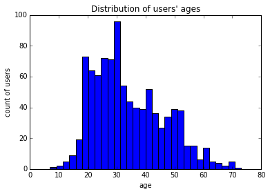
pandas' integration with matplotlib makes basic graphing of Series/DataFrames trivial. In this case, just call hist on the column to produce a histogram. We can also use matplotlib.pyplot to customize our graph a bit (always label your axes).
Binning our users
I don't think it'd be very useful to compare individual ages - let's bin our users into age groups using pandas.cut.
labels = ['0-9', '10-19', '20-29', '30-39', '40-49', '50-59', '60-69', '70-79']
lens['age_group'] = pd.cut(lens.age, range(0, 81, 10), right=False, labels=labels)
lens[['age', 'age_group']].drop_duplicates()[:10]
| age | age_group | |
|---|---|---|
| 0 | 60 | 60-69 |
| 397 | 21 | 20-29 |
| 459 | 33 | 30-39 |
| 524 | 30 | 30-39 |
| 782 | 23 | 20-29 |
| 995 | 29 | 20-29 |
| 1229 | 26 | 20-29 |
| 1664 | 31 | 30-39 |
| 1942 | 24 | 20-29 |
| 2270 | 32 | 30-39 |
pandas.cut allows you to bin numeric data. In the above lines, we first created labels to name our bins, then split our users into eight bins of ten years (0-9, 10-19, 20-29, etc.). Our use of right=False told the function that we wanted the bins to be exclusive of the max age in the bin (e.g. a 30 year old user gets the 30s label).
Now we can now compare ratings across age groups.
lens.groupby('age_group').agg({'rating': [np.size, np.mean]})
| rating | ||
|---|---|---|
| size | mean | |
| age_group | ||
| 0-9 | 43 | 3.767442 |
| 10-19 | 8181 | 3.486126 |
| 20-29 | 39535 | 3.467333 |
| 30-39 | 25696 | 3.554444 |
| 40-49 | 15021 | 3.591772 |
| 50-59 | 8704 | 3.635800 |
| 60-69 | 2623 | 3.648875 |
| 70-79 | 197 | 3.649746 |
Young users seem a bit more critical than other age groups. Let's look at how the 50 most rated movies are viewed across each age group. We can use the most_50 Series we created earlier for filtering.
lens.set_index('movie_id', inplace=True)
by_age = lens.loc[most_50.index].groupby(['title', 'age_group'])
by_age.rating.mean().head(15)
title                 age_group
Air Force One (1997)  10-19        3.647059
                      20-29        3.666667
                      30-39        3.570000
                      40-49        3.555556
                      50-59        3.750000
                      60-69        3.666667
                      70-79        3.666667
Alien (1979)          10-19        4.111111
                      20-29        4.026087
                      30-39        4.103448
                      40-49        3.833333
                      50-59        4.272727
                      60-69        3.500000
                      70-79        4.000000
Aliens (1986)         10-19        4.050000
Name: rating, dtype: float64
Notice that both the title and age group are indexes here, with the average rating value being a Series. This is going to produce a really long list of values.
Wouldn't it be nice to see the data as a table? Each title as a row, each age group as a column, and the average rating in each cell.
Behold! The magic of unstack!
by_age.rating.mean().unstack(1).fillna(0)[10:20]
| age_group | 0-9 | 10-19 | 20-29 | 30-39 | 40-49 | 50-59 | 60-69 | 70-79 |
|---|---|---|---|---|---|---|---|---|
| title | ||||||||
| E.T. the Extra-Terrestrial (1982) | 0 | 3.680000 | 3.609091 | 3.806818 | 4.160000 | 4.368421 | 4.375000 | 0.000000 |
| Empire Strikes Back, The (1980) | 4 | 4.642857 | 4.311688 | 4.052083 | 4.100000 | 3.909091 | 4.250000 | 5.000000 |
| English Patient, The (1996) | 5 | 3.739130 | 3.571429 | 3.621849 | 3.634615 | 3.774648 | 3.904762 | 4.500000 |
| Fargo (1996) | 0 | 3.937500 | 4.010471 | 4.230769 | 4.294118 | 4.442308 | 4.000000 | 4.333333 |
| Forrest Gump (1994) | 5 | 4.047619 | 3.785714 | 3.861702 | 3.847826 | 4.000000 | 3.800000 | 0.000000 |
| Fugitive, The (1993) | 0 | 4.320000 | 3.969925 | 3.981481 | 4.190476 | 4.240000 | 3.666667 | 0.000000 |
| Full Monty, The (1997) | 0 | 3.421053 | 4.056818 | 3.933333 | 3.714286 | 4.146341 | 4.166667 | 3.500000 |
| Godfather, The (1972) | 0 | 4.400000 | 4.345070 | 4.412844 | 3.929412 | 4.463415 | 4.125000 | 0.000000 |
| Groundhog Day (1993) | 0 | 3.476190 | 3.798246 | 3.786667 | 3.851064 | 3.571429 | 3.571429 | 4.000000 |
| Independence Day (ID4) (1996) | 0 | 3.595238 | 3.291429 | 3.389381 | 3.718750 | 3.888889 | 2.750000 | 0.000000 |
unstack, well, unstacks the specified level of a MultiIndex (by default, groupby turns the grouped field into an index - since we grouped by two fields, it became a MultiIndex). We unstacked the second index (remember that Python uses 0-based indexes), and then filled in NULL values with 0.
If we would have used:
by_age.rating.mean().unstack(0).fillna(0)
We would have had our age groups as rows and movie titles as columns.
Which movies do men and women most disagree on?
EDIT: I realized after writing this question that Wes McKinney basically went through the exact same question in his book. It's a good, yet simple example of pivot_table, so I'm going to leave it here. Seriously though, go buy the book.
Think about how you'd have to do this in SQL for a second. You'd have to use a combination of IF/CASE statements with aggregate functions in order to pivot your dataset. Your query would look something like this:
SELECT title, AVG(IF(sex = 'F', rating, NULL)), AVG(IF(sex = 'M', rating, NULL))
FROM lens
GROUP BY title;
Imagine how annoying it'd be if you had to do this on more than two columns.
DataFrame's have a pivot_table method that makes these kinds of operations much easier (and less verbose).
lens.reset_index('movie_id', inplace=True)
pivoted = lens.pivot_table(index=['movie_id', 'title'],
                           columns=['sex'],
                           values='rating',
                           fill_value=0)
pivoted.head()
| sex | F | M | |
|---|---|---|---|
| movie_id | title | ||
| 1 | Toy Story (1995) | 3.789916 | 3.909910 |
| 2 | GoldenEye (1995) | 3.368421 | 3.178571 |
| 3 | Four Rooms (1995) | 2.687500 | 3.108108 |
| 4 | Get Shorty (1995) | 3.400000 | 3.591463 |
| 5 | Copycat (1995) | 3.772727 | 3.140625 |
pivoted['diff'] = pivoted.M - pivoted.F
pivoted.head()
| sex | F | M | diff | |
|---|---|---|---|---|
| movie_id | title | |||
| 1 | Toy Story (1995) | 3.789916 | 3.909910 | 0.119994 |
| 2 | GoldenEye (1995) | 3.368421 | 3.178571 | -0.189850 |
| 3 | Four Rooms (1995) | 2.687500 | 3.108108 | 0.420608 |
| 4 | Get Shorty (1995) | 3.400000 | 3.591463 | 0.191463 |
| 5 | Copycat (1995) | 3.772727 | 3.140625 | -0.632102 |
pivoted.reset_index('movie_id', inplace=True)
disagreements = pivoted[pivoted.movie_id.isin(most_50.index)]['diff']
disagreements.sort_values().plot(kind='barh', figsize=[9, 15])
plt.title('Male vs. Female Avg. Ratings\n(Difference > 0 = Favored by Men)')
plt.ylabel('Title')
plt.xlabel('Average Rating Difference');
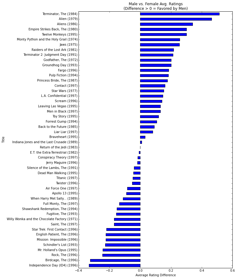
Of course men like Terminator more than women. Independence Day though? Really?
Additional Resources
- pandas documentation
- pandas videos from PyCon
- pandas and Python top 10
- Tom Augspurger's Modern pandas series
- Video from Tom's pandas tutorial at PyData Seattle 2015
Closing
This is the point where I finally wrap this tutorial up. Hopefully I've covered the basics well enough to pique your interest and help you get started with the library. If I've missed something critical, feel free to let me know on Twitter or in the comments - I'd love constructive feedback.